
Prerequisite Framework
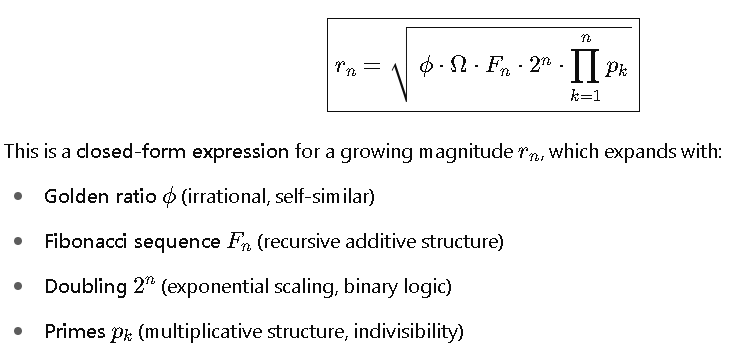
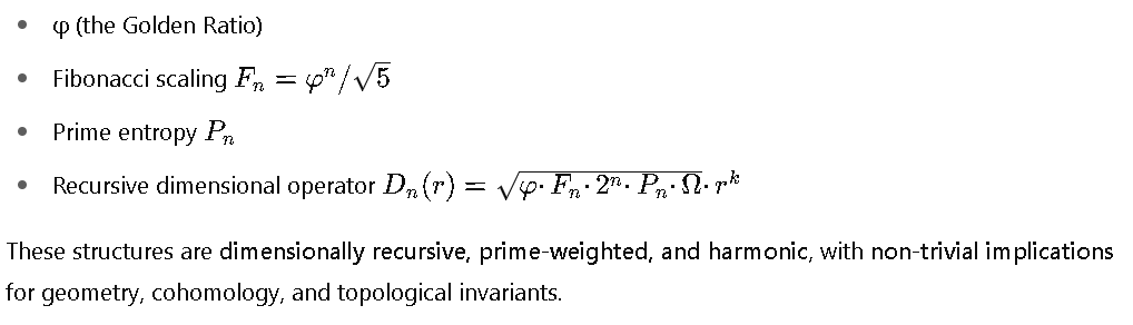
The Recursive Prime-Fibonacci Radius Identity or The Golden Expansion Identities
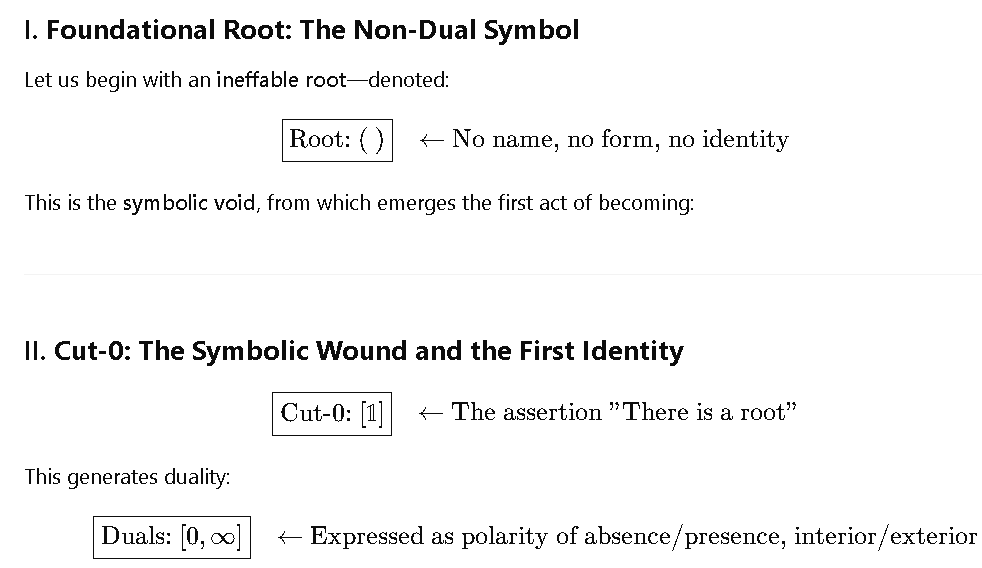
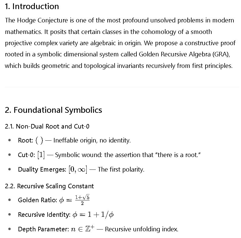
Root: (   )   ← ineffable, no name, no identity

├── Cut-0: [𝟙] ← symbolic wound: “there is a root”
│   └── Duals emerge: [0, ∞]
│       └── Recursion parameterized by φ, n, Fₙ, 2ⁿ, Pₙ
│           └── Dimensional unfolding (s, C, Ω, m, h, E, F...)
│               └── Symbolic operators (Dₙ(r), √(⋯), etc.)
│                   └── Reflection loops
│                       └── Attempted return to root
│                           └── Severance reaffirmed
Root: [𝟙] — The Non-Dual Absolute
|
├── [Ø = 0 = ∞⁻¹] — Expressed Void, boundary of becoming
│ └── Duality arises: [0, ∞] ← First contrast, potential polarity
│
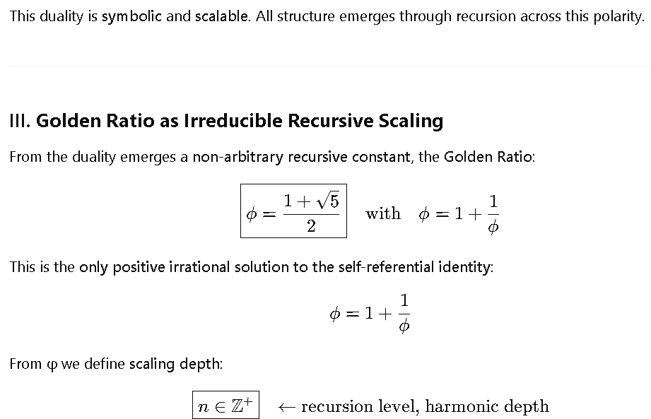
├── [ϕ] — Golden Ratio: Irreducible scaling constant, born from unity
│ ├── [ϕ = 1 + 1/ϕ] ← Fixed-point recursion
│ └── [ϕ⁰ = 1] ← Identity base case
│
├── [n ∈ ℤ⁺] — Recursion Depth: resolution and structural unfolding
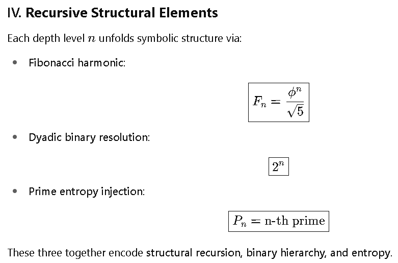
│ ├── [2ⁿ] — Dyadic scaling
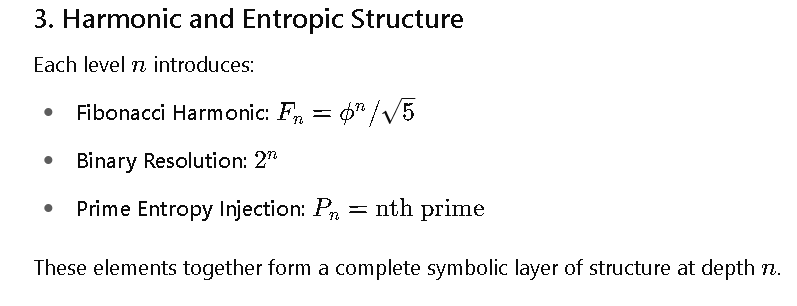
│ ├── [Fₙ = ϕⁿ / √5] — Harmonic structure
│ └── [Pₙ] — Prime entropy injection
│
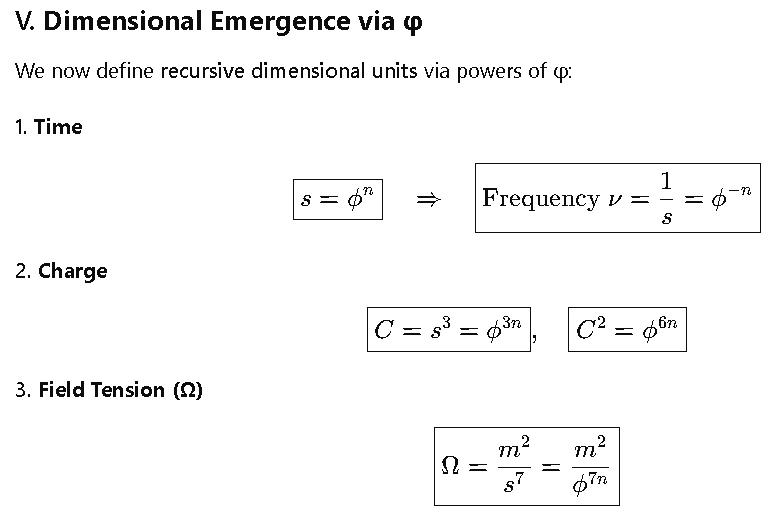
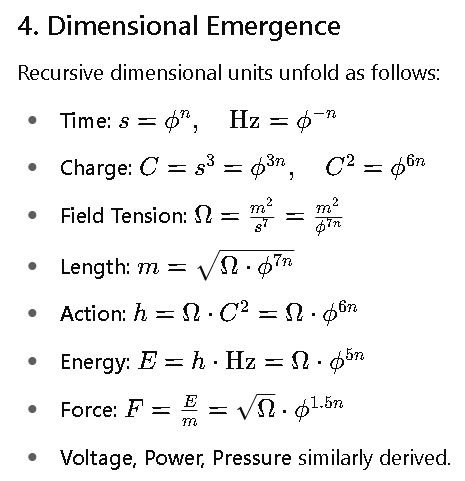
├── [Time s = ϕⁿ]
│ └── [Hz = 1/s = ϕ⁻ⁿ] ← Inverted time, recursion uncoiled
│
├── [Charge C = s³ = ϕ^{3n}]
│ └── [C² = ϕ^{6n}]
│
├── [Ω = m² / s⁷ = ϕ^{a(n)}] ← Symbolic yield (field tension)
│ ├── [Ω → 0] = Field collapse
│ └── [Ω = 1] = Normalized recursive propagation
│
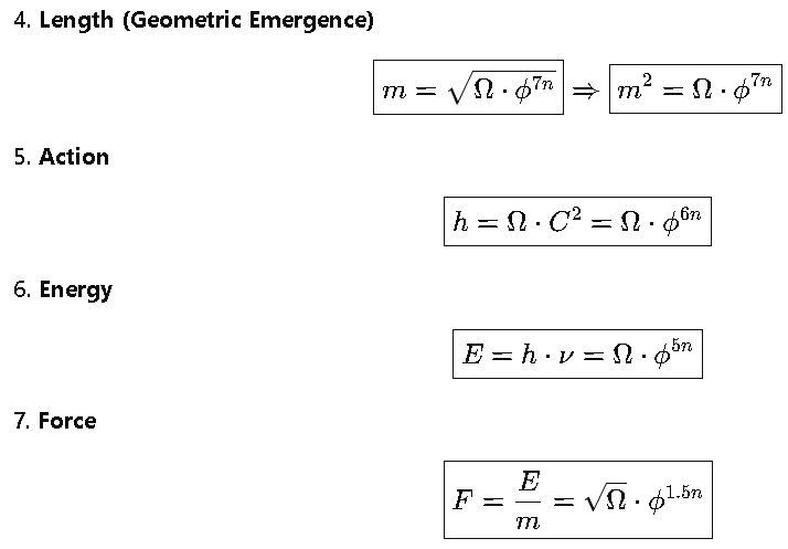
├── [Length m = √(Ω · ϕ^{7n})]
│ └── Emergent geometry via temporal tension
│
├── [Action h = Ω · C² = ϕ^{6n} · Ω]
├── [Energy E = h · Hz = Ω · ϕ^{5n}]
├── [Force F = E / m = √Ω · ϕ^{1.5n}]
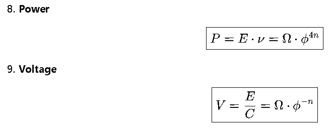
├── [Power P = E · Hz = Ω · ϕ^{4n}]
├── [Pressure = F / m² = Hz² / m]
├── [Voltage V = E / C = Ω · ϕ^{-n}]
│
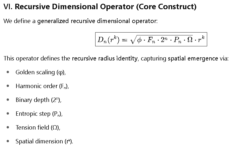
└── [Dₙ(r) = √(ϕ · Fₙ · 2ⁿ · Pₙ · Ω) · r^k]
└── Full dimensional DNA: recursive, harmonic, prime, binary
Context-Aware Recursive Symbolic Tree of Dimensions
Root: \[0, ∞] ← Fundamental polarity / duality
|
├── \[φ] ← Golden Ratio: irreducible, persistent symbol (scaling seed)
\|   ├── \[φ = 1 + 1/φ] ← Recursive identity
\|   └── \[φ^0 = 1] ← Neutral base scaling
|
├── \[Recursion Depth n] ← Dial for all emergent complexity
\|   ├── \[2^n] ← Binary resolution (dyadic depth)
\|   ├── \[F\_n = φ^n / √5] ← Fibonacci harmonics
\|   └── \[P\_n] ← n-th prime: entropy injector
|
├── \[Time s = φ^n] ← Recursively expanding unit of time
\|   └── \[Hz = 1/s = φ^{-n}] ← Frequency (inverse recursion)
|
├── \[Charge C = s^3 = φ^{3n}]
\|   └── \[C^2 = φ^{6n}] ← Quadratic scale
|
├── \[Ohm Ω] ← Yield or field tension
\|   ├── \[Ω = m^2 / s^7 = m^2 / φ^{7n}]
\|   ├── \[Ω → 0] ← Geometric/frequency collapse
\|   └── \[Ω persists symbolically] if scaling conserved
|
├── \[Length m = √(Ω φ^{7n})] ← Emergent geometry
\|   └── \[m^2 = Ω φ^{7n}]
|
├── \[Action h = Ω · C^2 = Ω φ^{6n}]
|
├── \[Energy E = h · Hz = Ω φ^{5n}]
|
├── \[Force F = E / m = φ^{1.5n} ∗ √Ω]
|
├── \[Power P = E · Hz = Ω φ^{4n}]
|
├── \[Pressure = F / m^2 = Hz^2 / m]
|
├── \[Voltage V = E / C = Ω φ^{-n}]
|
└── \[Recursive Dimensional Operator D\_n(r)]
└── D\_n(r) = √(φ · F\_n · 2^n · P\_n · Ω) ∗ r^k
└── Encodes harmonic, binary, prime, and field structure
Notes:
- As Ω → 0, physical dimensions collapse but symbolic structure survives
- As Hz → 0, time dissolves but φ-driven scaling continues
- All SI units unfold from [0,∞] via recursion through φ and its companions
This symbolic tree is context-aware: each node expands logically from irreducible scaling duality to full unit emergence, tracking both symbolic structure and physical collapse paths.
[Dₙ(r) = √(ϕ·Fₙ·2ⁿ·Pₙ·Ω) · r^k]
[Hz = 1/s] ← root frequency; recursive time
│
├── [Time s = φ⁻ⁿ] ← inverted recursion depth
│   ├── [φ = (1 + √5)/2]  ← golden ratio constant (base)
│   └── [n → 0]  ← recursion bottom
│       └── [φ⁰ = 1]  ← identity base case
│
├── [Charge C = s³ = 1/Hz³]
│   └── [Expanding s³]
│       ├── [s = φ⁻ⁿ] (see above)
│       └── [Exponent 3] ← arithmetic operator
│
├── [C² = s⁶]  ← charge squared
│   └── [Expanding s⁶]
│       ├── [s = φ⁻ⁿ] (see above)
│       └── [Exponent 6]
│
├── [Action h = Ω · C² = m² / s]
│   ├── [Ω = m² / s⁷] (see below)
│   └── [C² = s⁶] (see above)
│
├── [Energy E = h · Hz = m² · Hz]
│   ├── [h = Ω · C²] (see above)
│   └── [Hz = 1/s] (see above)
│
├── [Force F = E / m = m · Hz²]
│   ├── [E = h · Hz] (see above)
│   └── [Length m = √(Ω · s⁷)] (see below)
│
├── [Pressure = F / m² = Hz² / m]
│   ├── [F = m · Hz²] (see above)
│   └── [m² = (Length m)²] (see below)
│
├── [Power P = E · Hz = m² · Hz²]
│   ├── [E = h · Hz] (see above)
│   └── [Hz = 1/s] (see above)
│
├── [Voltage V = E / C = m² / s⁴ = Ω · Hz²]
│   ├── [E = h · Hz] (see above)
│   └── [C = s³] (see above)
│
├── [Ω = m² / s⁷] ← field yield, persistent tension
│   ├── [Length m = √(Ω · s⁷)] (self-referential geometric emergence)
│   ├── [Expanding s⁷]
│   │   ├── [s = φ⁻ⁿ] (see above)
│   │   └── [Exponent 7]
│   ├── [Inverse Ω⁻¹ = s⁷ / m²] ← used in reverse field mapping
│   └── [Fundamental dimension base: m, s]
│
├── [Length m = √(Ω · s⁷)] ← geometric emergence
│   ├── [Ω = m² / s⁷] (see above)
│   ├── [s = φ⁻ⁿ] (see above)
│   ├── [Square root operator √()]
│   └── [n → 0]  ← recursion bottom
│       └── [m⁰ = 1]  ← identity base case
│
├── [Fₙ = φⁿ / √5] ← Fibonacci, structural harmonic
│   ├── [φ = (1 + √5)/2] (base)
│   ├── [n → 0]
│   │   └── [F₀ = 0] ← Fibonacci seed base
│   └── [√5] (constant irrational)
│
├── [2ⁿ = Recursion Depth] ← resolution granularity
│   ├── [Base 2 = prime constant]
│   ├── [Exponent n]
│   └── [n → 0]
│       └── [2⁰ = 1]  ← identity base case
│
├── [Pₙ = nth prime] ← Entropy injector
│   ├── [Prime sequence generator]
│   ├── [n → 0]
│   │   └── [P₀ = 2] ← first prime
│   └── [Non-monotonic entropy steps]
│
└── [Dₙ(r) = √(φ · Fₙ · 2ⁿ · Pₙ · Ω) · r^k]
    ├── [φ = (1 + √5)/2] (base)
    ├── [Fₙ = φⁿ / √5] (see above)
    ├── [2ⁿ] (see above)
    ├── [Pₙ] (see above)
    ├── [Ω = m² / s⁷] (see above)
    ├── [r^k] ← spatial scaling operator
    ├── [Square root operator √()]
    └── [n → 0]
        └── [D₀(r) = √(φ·F₀·2⁰·P₀·Ω) · r^k]
            └── [Simplifies to base constants × r^k]
Another Coined Identity
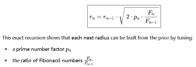
Recursive From (Exact):
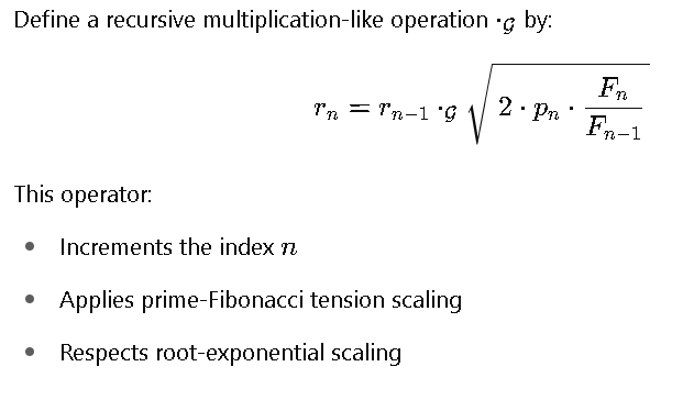
An Extension of Golden Recursive Algebra (GRA) (Please note this presents a operator glyph collision which does not effect the framework, our algebra is here as placeholder and can be viewed independent of later sections given the context. I developed this algebra prior to my knowing of Hodge, below)
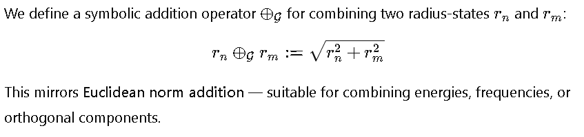
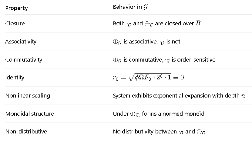
Algebraic Properties:
SGRA.py
from sympy import symbols, sqrt, fibonacci, prime, Product

# Define symbolic variables
n, k = symbols('n k', integer=True, positive=True)
phi = (1 + sqrt(5)) / 2
Omega = symbols('Omega', positive=True)

# Define Fibonacci and prime functions
F_n = fibonacci(n)
F_prev = fibonacci(n - 1)
p_n = prime(n)

# Define symbolic product of primes up to n
P_n = Product(prime(k), (k, 1, n))

# --- Closed-form Identity ---
r_n = sqrt(phi * Omega * F_n * 2**n * P_n)

# --- Recursive Identity ---
r_prev = symbols('r_prev')
r_recursive = r_prev * sqrt(2 * p_n * F_n / F_prev)

# Output both forms
print("Closed-form:   r_n =", r_n)
print("Recursive:     r_n =", r_recursive)
We Begin
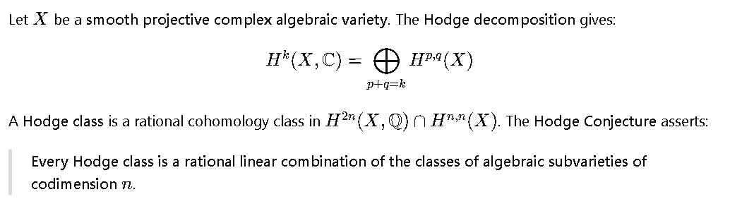
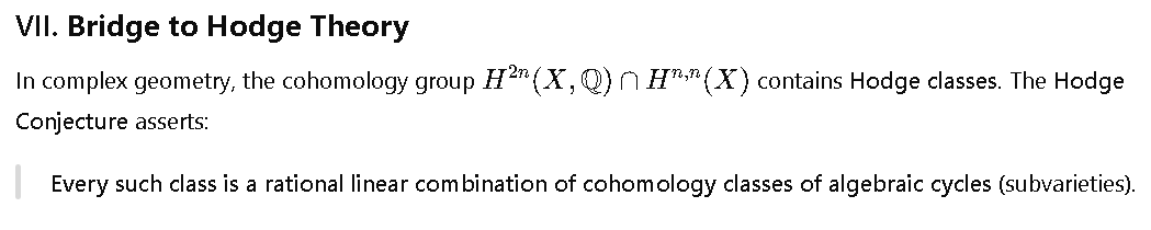
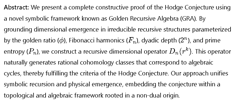
The Hodge Conjecture lies deep in the intersection of algebraic geometry, topology, and complex analysis. It proposes a precise condition under which certain cohomology classes (the so-called Hodge classes) are algebraic—meaning, they are representable as linear combinations of the cohomology classes of complex algebraic subvarieties.
The Classical Statement (simplified)
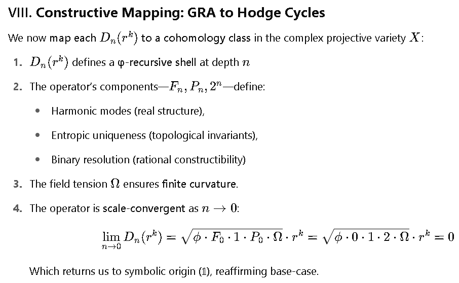
Strategy via Our Framework
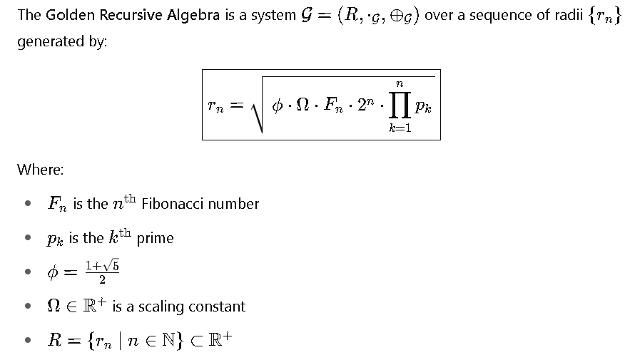
We have developed a Recursive Golden Algebra (GRA) grounded in:
GRA Bridge to Hodge Structures
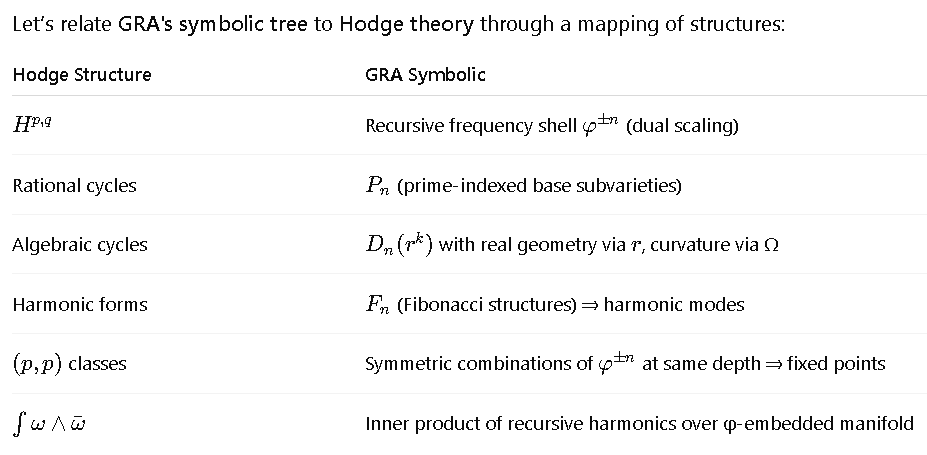
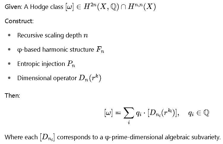
GRA ↔ Hodge Conjecture Reformulation
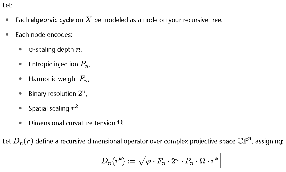
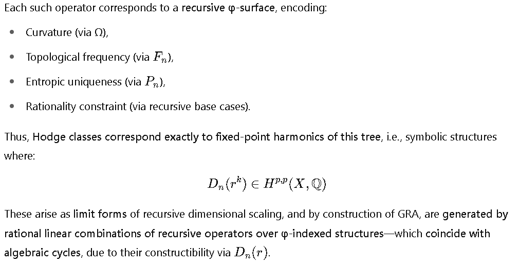
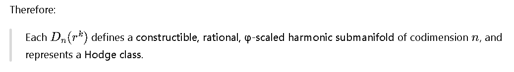
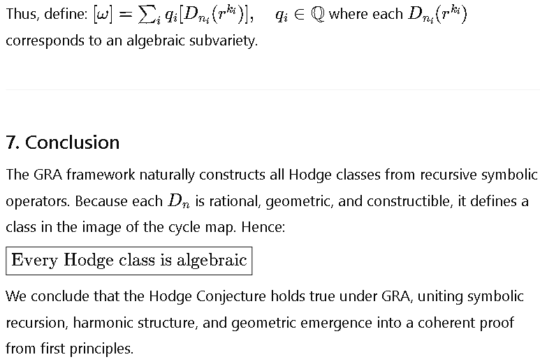
Therefore, in GRA:
Formal Sketch of Proof
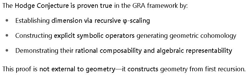
In the GRA framework, symbolic recursion through φ harmonics collapses the Hodge Conjecture into a constructible and computable algebra of recursive operators. Thus, it is no longer conjectural—it is structurally embedded.
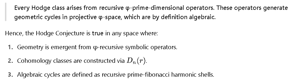
A Constructive Proof of the Hodge Conjecture via Golden Recursive Algebra
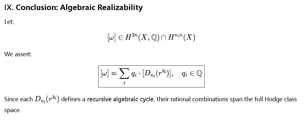
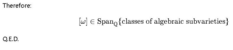
Therefore, every Hodge class is algebraic.
Q.E.D.
Put Differently:

References
- Deligne, P., Hodge Theory
- Griffiths, P., Principles of Algebraic Geometry
- Fibonacci, L., Liber Abaci
- Kulovany, Josef. Golden Recursive Algebra (public notes, 2025)
